Sea Surface Altimetry Data Analysis¶

Example on using the gridded sea-surface altimetry data from The Copernicus Marine Environment

http://marine.copernicus.eu/services-portfolio/access-to-products/?option=com_csw&view=details&product_id=SEALEVEL_GLO_PHY_L4_REP_OBSERVATIONS_008_047

This is a widely used dataset in physical oceanography and climate.

globe image

The dataset has already been extracted from copernicus and stored in google cloud storage in xarray-zarr format.

import numpy as np
import xarray as xr
import matplotlib.pyplot as plt
import gcsfs
plt.rcParams['figure.figsize'] = (15,10)

Initialize Dataset¶

Here we load the dataset from the zarr store. Note that this very large dataset initializes nearly instantly, and we can see the full list of variables and coordinates.

gcsmap = gcsfs.mapping.GCSMap('pangeo-data/dataset-duacs-rep-global-merged-allsat-phy-l4-v3-alt')
ds = xr.open_zarr(gcsmap)
ds

<xarray.Dataset>
Dimensions:    (latitude: 720, longitude: 1440, nv: 2, time: 8901)
Coordinates:
    crs        int32 ...
    lat_bnds   (time, latitude, nv) float32 dask.array<shape=(8901, 720, 2), chunksize=(5, 720, 2)>
  * latitude   (latitude) float32 -89.875 -89.625 -89.375 -89.125 -88.875 ...
    lon_bnds   (longitude, nv) float32 dask.array<shape=(1440, 2), chunksize=(1440, 2)>
  * longitude  (longitude) float32 0.125 0.375 0.625 0.875 1.125 1.375 1.625 ...
  * nv         (nv) int32 0 1
  * time       (time) datetime64[ns] 1993-01-01 1993-01-02 1993-01-03 ...
Data variables:
    adt        (time, latitude, longitude) float64 dask.array<shape=(8901, 720, 1440), chunksize=(5, 720, 1440)>
    err        (time, latitude, longitude) float64 dask.array<shape=(8901, 720, 1440), chunksize=(5, 720, 1440)>
    sla        (time, latitude, longitude) float64 dask.array<shape=(8901, 720, 1440), chunksize=(5, 720, 1440)>
    ugos       (time, latitude, longitude) float64 dask.array<shape=(8901, 720, 1440), chunksize=(5, 720, 1440)>
    ugosa      (time, latitude, longitude) float64 dask.array<shape=(8901, 720, 1440), chunksize=(5, 720, 1440)>
    vgos       (time, latitude, longitude) float64 dask.array<shape=(8901, 720, 1440), chunksize=(5, 720, 1440)>
    vgosa      (time, latitude, longitude) float64 dask.array<shape=(8901, 720, 1440), chunksize=(5, 720, 1440)>
Attributes:
    Conventions:                     CF-1.6
    Metadata_Conventions:            Unidata Dataset Discovery v1.0
    cdm_data_type:                   Grid
    comment:                         Sea Surface Height measured by Altimetry...
    contact:                         servicedesk.cmems@mercator-ocean.eu
    creator_email:                   servicedesk.cmems@mercator-ocean.eu
    creator_name:                    CMEMS - Sea Level Thematic Assembly Center
    creator_url:                     http://marine.copernicus.eu
    date_created:                    2014-02-26T16:09:13Z
    date_issued:                     2014-01-06T00:00:00Z
    date_modified:                   2015-11-10T19:42:51Z
    geospatial_lat_max:              89.875
    geospatial_lat_min:              -89.875
    geospatial_lat_resolution:       0.25
    geospatial_lat_units:            degrees_north
    geospatial_lon_max:              359.875
    geospatial_lon_min:              0.125
    geospatial_lon_resolution:       0.25
    geospatial_lon_units:            degrees_east
    geospatial_vertical_max:         0.0
    geospatial_vertical_min:         0.0
    geospatial_vertical_positive:    down
    geospatial_vertical_resolution:  point
    geospatial_vertical_units:       m
    history:                         2014-02-26T16:09:13Z: created by DUACS D...
    institution:                     CLS, CNES
    keywords:                        Oceans > Ocean Topography > Sea Surface ...
    keywords_vocabulary:             NetCDF COARDS Climate and Forecast Stand...
    license:                         http://marine.copernicus.eu/web/27-servi...
    platform:                        ERS-1, Topex/Poseidon
    processing_level:                L4
    product_version:                 5.0
    project:                         COPERNICUS MARINE ENVIRONMENT MONITORING...
    references:                      http://marine.copernicus.eu
    source:                          Altimetry measurements
    ssalto_duacs_comment:            The reference mission used for the altim...
    standard_name_vocabulary:        NetCDF Climate and Forecast (CF) Metadat...
    summary:                         SSALTO/DUACS Delayed-Time Level-4 sea su...
    time_coverage_duration:          P1D
    time_coverage_end:               1993-01-01T12:00:00Z
    time_coverage_resolution:        P1D
    time_coverage_start:             1992-12-31T12:00:00Z
    title:                           DT merged all satellites Global Ocean Gr...

Examine Metadata¶

For those unfamiliar with this dataset, the variable metadata is very helpful for understanding what the variables actually represent

for v in ds.data_vars:
    print('{:>10}: {}'.format(v, ds[v].attrs['long_name']))

  adt: Absolute dynamic topography
  err: Formal mapping error
  sla: Sea level anomaly
 ugos: Absolute geostrophic velocity: zonal component
ugosa: Geostrophic velocity anomalies: zonal component
 vgos: Absolute geostrophic velocity: meridian component
vgosa: Geostrophic velocity anomalies: meridian component

Create and Connect to Dask Distributed Cluster¶

from dask.distributed import Client, progress

from dask_kubernetes import KubeCluster
cluster = KubeCluster(n_workers=20)
cluster

VBox(children=(HTML(value='<h2>KubeCluster</h2>'), HBox(children=(HTML(value='n<div>n  <style scoped>n    .…

** ☝️ Don’t forget to click the link above to view the scheduler dashboard! **

client = Client(cluster)
client

Client

Scheduler: tcp://10.21.61.9:44494
Dashboard: /user/rabernat/proxy/8787/status

Cluster

Workers: 20
Cores: 40
Memory: 440.00 GB

Visually Examine Some of the Data¶

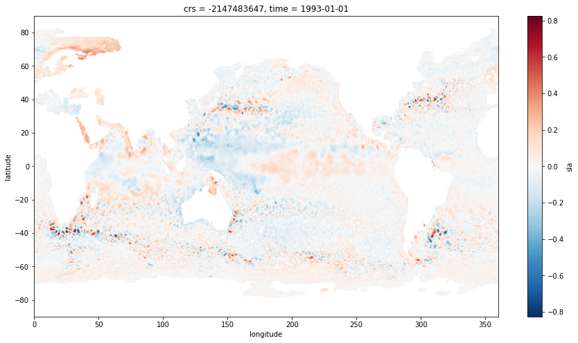
Let’s do a sanity check that the data looks reasonable:

plt.rcParams['figure.figsize'] = (15, 8)
ds.sla.sel(time='1982-08-07', method='nearest').plot()

<matplotlib.collections.QuadMesh at 0x7f83ecf44550>

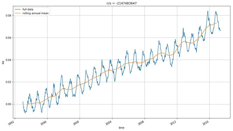
Timeseries of Global Mean Sea Level¶

Here we make a simple yet fundamental calculation: the rate of increase of global mean sea level over the observational period.

# the number of GB involved in the reduction
ds.sla.nbytes/1e9

73.8284544

# the computationally intensive step
sla_timeseries = ds.sla.mean(dim=('latitude', 'longitude')).load()

sla_timeseries.plot(label='full data')
sla_timeseries.rolling(time=365, center=True).mean().plot(label='rolling annual mean')
plt.legend()
plt.grid()

Astute readers will note that this global mean is biased because the pixels were averaged naively, neglecting the spherical geometry of Earth. Below we repeat with a proper a weighing factor based on cosine of latitude.

coslat = np.cos(np.deg2rad(ds.latitude)).where(~ds.sla.isnull())
weights = coslat / coslat.sum(dim=('latitude', 'longitude'))
sla_timeseries_weighted = (ds.sla * weights).sum(dim=('latitude', 'longitude'))
sla_timeseries_weighted.load()

<xarray.DataArray (time: 8901)>
array([-0.000846, -0.00104 , -0.001204, ...,  0.070539,  0.070415,  0.070242])
Coordinates:
    crs      int32 -2147483647
  * time     (time) datetime64[ns] 1993-01-01 1993-01-02 1993-01-03 ...

sla_timeseries.rolling(time=365, center=True).mean().plot(label='unweighted')
sla_timeseries_weighted.rolling(time=365, center=True).mean().plot(label='weighted')
plt.legend()
plt.grid()

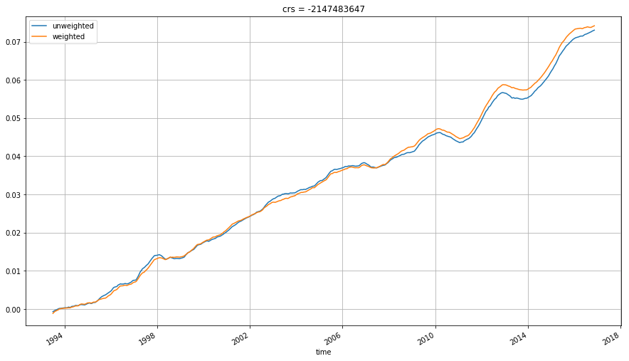
In this case, the weighting actually didn’t make much difference!

In order to understand how the sea level rise is distributed in latitude, we can make a sort of Hovmöller diagram.

sla_hov = ds.sla.mean(dim='longitude').load()

fig, ax = plt.subplots(figsize=(12,4))
sla_hov.transpose().plot(vmax=0.2, ax=ax)

<matplotlib.collections.QuadMesh at 0x7f83e07d8320>

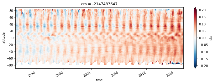
We can see that most sea level rise is actually in the Southern Hemisphere.

Sea Level Variability¶

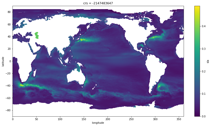
We can quantify the natural variability in sea level by looking at its standard deviation in time. (We have not bothered to remove the trend; in this case, the trend is much smaller than the interannual variability.)

sla_std = ds.sla.std(dim='time').load()

sla_std.plot()

<matplotlib.collections.QuadMesh at 0x7f83e03a9b00>

Download python script: sea-surface-height.py

Download Jupyter notebook: sea-surface-height.ipynb