
- Blog
- Site
- Page
- « Sea Surface A...
- Climate modeling »
Evaluating the conservation of heat and salt content in the Southern Ocean State Estimate
Author: Ryan Abernathey

SOSE Logo
Below we create a dask cluster with 30 nodes to do our work for us.
from dask.distributed import Client, progress
from dask_kubernetes import KubeCluster
cluster = KubeCluster(n_workers=50)
cluster
VBox(children=(HTML(value='<h2>KubeCluster</h2>'), HBox(children=(HTML(value='n<div>n <style scoped>n .…
** ☝️ don’t forget to follow along on the dashboard **
client = Client(cluster)
client
Client
|
Cluster
|
Import necessary Python packages
import xarray as xr
from matplotlib import pyplot as plt
import gcsfs
import dask
import dask.array as dsa
import numpy as np
ds = xr.open_zarr(gcsfs.GCSMap('pangeo-data/SOSE'))
ds
<xarray.Dataset>
Dimensions:   (XC: 2160, XG: 2160, YC: 320, YG: 320, Z: 42, Zl: 42, Zp1: 43, Zu: 42, time: 438)
Coordinates:
    Depth     (YC, XC) float32 dask.array<shape=(320, 2160), chunksize=(320, 2160)>
    PHrefC    (Z) float32 dask.array<shape=(42,), chunksize=(42,)>
    PHrefF    (Zp1) float32 dask.array<shape=(43,), chunksize=(43,)>
  * XC        (XC) float32 0.083333336 0.25 0.4166667 0.5833334 0.75 ...
  * XG        (XG) float32 5.551115e-17 0.16666667 0.33333334 0.5 0.6666667 ...
  * YC        (YC) float32 -77.87497 -77.7083 -77.54163 -77.37497 -77.2083 ...
  * YG        (YG) float32 -77.9583 -77.79163 -77.62497 -77.4583 -77.29163 ...
  * Z         (Z) float32 -5.0 -15.5 -27.0 -39.5 -53.0 -68.0 -85.0 -104.0 ...
  * Zl        (Zl) float32 0.0 -10.0 -21.0 -33.0 -46.0 -60.0 -76.0 -94.0 ...
  * Zp1       (Zp1) float32 0.0 -10.0 -21.0 -33.0 -46.0 -60.0 -76.0 -94.0 ...
  * Zu        (Zu) float32 -10.0 -21.0 -33.0 -46.0 -60.0 -76.0 -94.0 -114.0 ...
    drC       (Zp1) float32 dask.array<shape=(43,), chunksize=(43,)>
    drF       (Z) float32 dask.array<shape=(42,), chunksize=(42,)>
    dxC       (YC, XG) float32 dask.array<shape=(320, 2160), chunksize=(320, 2160)>
    dxG       (YG, XC) float32 dask.array<shape=(320, 2160), chunksize=(320, 2160)>
    dyC       (YG, XC) float32 dask.array<shape=(320, 2160), chunksize=(320, 2160)>
    dyG       (YC, XG) float32 dask.array<shape=(320, 2160), chunksize=(320, 2160)>
    hFacC     (Z, YC, XC) float32 dask.array<shape=(42, 320, 2160), chunksize=(42, 320, 2160)>
    hFacS     (Z, YG, XC) float32 dask.array<shape=(42, 320, 2160), chunksize=(42, 320, 2160)>
    hFacW     (Z, YC, XG) float32 dask.array<shape=(42, 320, 2160), chunksize=(42, 320, 2160)>
    iter      (time) int64 dask.array<shape=(438,), chunksize=(438,)>
    rA        (YC, XC) float32 dask.array<shape=(320, 2160), chunksize=(320, 2160)>
    rAs       (YG, XC) float32 dask.array<shape=(320, 2160), chunksize=(320, 2160)>
    rAw       (YC, XG) float32 dask.array<shape=(320, 2160), chunksize=(320, 2160)>
    rAz       (YG, XG) float32 dask.array<shape=(320, 2160), chunksize=(320, 2160)>
  * time      (time) datetime64[ns] 2005-01-06 2005-01-11 2005-01-16 ...
Data variables:
    ADVr_SLT  (time, Zl, YC, XC) float32 dask.array<shape=(438, 42, 320, 2160), chunksize=(1, 42, 320, 2160)>
    ADVr_TH   (time, Zl, YC, XC) float32 dask.array<shape=(438, 42, 320, 2160), chunksize=(1, 42, 320, 2160)>
    ADVx_SLT  (time, Z, YC, XG) float32 dask.array<shape=(438, 42, 320, 2160), chunksize=(1, 42, 320, 2160)>
    ADVx_TH   (time, Z, YC, XG) float32 dask.array<shape=(438, 42, 320, 2160), chunksize=(1, 42, 320, 2160)>
    ADVy_SLT  (time, Z, YG, XC) float32 dask.array<shape=(438, 42, 320, 2160), chunksize=(1, 42, 320, 2160)>
    ADVy_TH   (time, Z, YG, XC) float32 dask.array<shape=(438, 42, 320, 2160), chunksize=(1, 42, 320, 2160)>
    DFrE_SLT  (time, Zl, YC, XC) float32 dask.array<shape=(438, 42, 320, 2160), chunksize=(1, 42, 320, 2160)>
    DFrE_TH   (time, Zl, YC, XC) float32 dask.array<shape=(438, 42, 320, 2160), chunksize=(1, 42, 320, 2160)>
    DFrI_SLT  (time, Zl, YC, XC) float32 dask.array<shape=(438, 42, 320, 2160), chunksize=(1, 42, 320, 2160)>
    DFrI_TH   (time, Zl, YC, XC) float32 dask.array<shape=(438, 42, 320, 2160), chunksize=(1, 42, 320, 2160)>
    DFxE_SLT  (time, Z, YC, XG) float32 dask.array<shape=(438, 42, 320, 2160), chunksize=(1, 42, 320, 2160)>
    DFxE_TH   (time, Z, YC, XG) float32 dask.array<shape=(438, 42, 320, 2160), chunksize=(1, 42, 320, 2160)>
    DFyE_SLT  (time, Z, YG, XC) float32 dask.array<shape=(438, 42, 320, 2160), chunksize=(1, 42, 320, 2160)>
    DFyE_TH   (time, Z, YG, XC) float32 dask.array<shape=(438, 42, 320, 2160), chunksize=(1, 42, 320, 2160)>
    DRHODR    (time, Zl, YC, XC) float32 dask.array<shape=(438, 42, 320, 2160), chunksize=(1, 42, 320, 2160)>
    ETAN      (time, YC, XC) float32 dask.array<shape=(438, 320, 2160), chunksize=(1, 320, 2160)>
    EXFswnet  (time, YC, XC) float32 dask.array<shape=(438, 320, 2160), chunksize=(1, 320, 2160)>
    KPPg_SLT  (time, Zl, YC, XC) float32 dask.array<shape=(438, 42, 320, 2160), chunksize=(1, 42, 320, 2160)>
    KPPg_TH   (time, Zl, YC, XC) float32 dask.array<shape=(438, 42, 320, 2160), chunksize=(1, 42, 320, 2160)>
    PHIHYD    (time, Z, YC, XC) float32 dask.array<shape=(438, 42, 320, 2160), chunksize=(1, 42, 320, 2160)>
    SALT      (time, Z, YC, XC) float32 dask.array<shape=(438, 42, 320, 2160), chunksize=(1, 42, 320, 2160)>
    SFLUX     (time, YC, XC) float32 dask.array<shape=(438, 320, 2160), chunksize=(1, 320, 2160)>
    SIarea    (time, YC, XC) float32 dask.array<shape=(438, 320, 2160), chunksize=(1, 320, 2160)>
    SIatmFW   (time, YC, XC) float32 dask.array<shape=(438, 320, 2160), chunksize=(1, 320, 2160)>
    SIatmQnt  (time, YC, XC) float32 dask.array<shape=(438, 320, 2160), chunksize=(1, 320, 2160)>
    SIdHbATC  (time, YC, XC) float32 dask.array<shape=(438, 320, 2160), chunksize=(1, 320, 2160)>
    SIdHbATO  (time, YC, XC) float32 dask.array<shape=(438, 320, 2160), chunksize=(1, 320, 2160)>
    SIdHbOCN  (time, YC, XC) float32 dask.array<shape=(438, 320, 2160), chunksize=(1, 320, 2160)>
    SIdSbATC  (time, YC, XC) float32 dask.array<shape=(438, 320, 2160), chunksize=(1, 320, 2160)>
    SIdSbOCN  (time, YC, XC) float32 dask.array<shape=(438, 320, 2160), chunksize=(1, 320, 2160)>
    SIempmr   (time, YC, XC) float32 dask.array<shape=(438, 320, 2160), chunksize=(1, 320, 2160)>
    SIfu      (time, YC, XG) float32 dask.array<shape=(438, 320, 2160), chunksize=(1, 320, 2160)>
    SIfv      (time, YG, XC) float32 dask.array<shape=(438, 320, 2160), chunksize=(1, 320, 2160)>
    SIheff    (time, YC, XC) float32 dask.array<shape=(438, 320, 2160), chunksize=(1, 320, 2160)>
    SIhsnow   (time, YC, XC) float32 dask.array<shape=(438, 320, 2160), chunksize=(1, 320, 2160)>
    SIsnPrcp  (time, YC, XC) float32 dask.array<shape=(438, 320, 2160), chunksize=(1, 320, 2160)>
    SItflux   (time, YC, XC) float32 dask.array<shape=(438, 320, 2160), chunksize=(1, 320, 2160)>
    SIuheff   (time, YC, XG) float32 dask.array<shape=(438, 320, 2160), chunksize=(1, 320, 2160)>
    SIuice    (time, YC, XG) float32 dask.array<shape=(438, 320, 2160), chunksize=(1, 320, 2160)>
    SIvheff   (time, YG, XC) float32 dask.array<shape=(438, 320, 2160), chunksize=(1, 320, 2160)>
    SIvice    (time, YG, XC) float32 dask.array<shape=(438, 320, 2160), chunksize=(1, 320, 2160)>
    TFLUX     (time, YC, XC) float32 dask.array<shape=(438, 320, 2160), chunksize=(1, 320, 2160)>
    THETA     (time, Z, YC, XC) float32 dask.array<shape=(438, 42, 320, 2160), chunksize=(1, 42, 320, 2160)>
    TOTSTEND  (time, Z, YC, XC) float32 dask.array<shape=(438, 42, 320, 2160), chunksize=(1, 42, 320, 2160)>
    TOTTTEND  (time, Z, YC, XC) float32 dask.array<shape=(438, 42, 320, 2160), chunksize=(1, 42, 320, 2160)>
    UVEL      (time, Z, YC, XG) float32 dask.array<shape=(438, 42, 320, 2160), chunksize=(1, 42, 320, 2160)>
    VVEL      (time, Z, YG, XC) float32 dask.array<shape=(438, 42, 320, 2160), chunksize=(1, 42, 320, 2160)>
    WSLTMASS  (time, Zl, YC, XC) float32 dask.array<shape=(438, 42, 320, 2160), chunksize=(1, 42, 320, 2160)>
    WTHMASS   (time, Zl, YC, XC) float32 dask.array<shape=(438, 42, 320, 2160), chunksize=(1, 42, 320, 2160)>
    WVEL      (time, Zl, YC, XC) float32 dask.array<shape=(438, 42, 320, 2160), chunksize=(1, 42, 320, 2160)>
    oceFreez  (time, YC, XC) float32 dask.array<shape=(438, 320, 2160), chunksize=(1, 320, 2160)>
    oceQsw    (time, YC, XC) float32 dask.array<shape=(438, 320, 2160), chunksize=(1, 320, 2160)>
    oceTAUX   (time, YC, XG) float32 dask.array<shape=(438, 320, 2160), chunksize=(1, 320, 2160)>
    oceTAUY   (time, YG, XC) float32 dask.array<shape=(438, 320, 2160), chunksize=(1, 320, 2160)>
    surForcS  (time, YC, XC) float32 dask.array<shape=(438, 320, 2160), chunksize=(1, 320, 2160)>
    surForcT  (time, YC, XC) float32 dask.array<shape=(438, 320, 2160), chunksize=(1, 320, 2160)>
print('Total Size: %6.2F GB' % (ds.nbytes / 1e9))
Total Size: 1408.75 GB
A trick for optimization: split the dataset into coordinates and data variables, and then drop the coordinates from the data variables. This makes it easier to align the data variables in arithmetic operations.
coords = ds.coords.to_dataset().reset_coords()
dsr = ds.reset_coords(drop=True)
dsr
<xarray.Dataset>
Dimensions:   (XC: 2160, XG: 2160, YC: 320, YG: 320, Z: 42, Zl: 42, Zp1: 43, Zu: 42, time: 438)
Coordinates:
  * XC        (XC) float32 0.083333336 0.25 0.4166667 0.5833334 0.75 ...
  * XG        (XG) float32 5.551115e-17 0.16666667 0.33333334 0.5 0.6666667 ...
  * YC        (YC) float32 -77.87497 -77.7083 -77.54163 -77.37497 -77.2083 ...
  * YG        (YG) float32 -77.9583 -77.79163 -77.62497 -77.4583 -77.29163 ...
  * Z         (Z) float32 -5.0 -15.5 -27.0 -39.5 -53.0 -68.0 -85.0 -104.0 ...
  * Zl        (Zl) float32 0.0 -10.0 -21.0 -33.0 -46.0 -60.0 -76.0 -94.0 ...
  * Zp1       (Zp1) float32 0.0 -10.0 -21.0 -33.0 -46.0 -60.0 -76.0 -94.0 ...
  * Zu        (Zu) float32 -10.0 -21.0 -33.0 -46.0 -60.0 -76.0 -94.0 -114.0 ...
  * time      (time) datetime64[ns] 2005-01-06 2005-01-11 2005-01-16 ...
Data variables:
    ADVr_SLT  (time, Zl, YC, XC) float32 dask.array<shape=(438, 42, 320, 2160), chunksize=(1, 42, 320, 2160)>
    ADVr_TH   (time, Zl, YC, XC) float32 dask.array<shape=(438, 42, 320, 2160), chunksize=(1, 42, 320, 2160)>
    ADVx_SLT  (time, Z, YC, XG) float32 dask.array<shape=(438, 42, 320, 2160), chunksize=(1, 42, 320, 2160)>
    ADVx_TH   (time, Z, YC, XG) float32 dask.array<shape=(438, 42, 320, 2160), chunksize=(1, 42, 320, 2160)>
    ADVy_SLT  (time, Z, YG, XC) float32 dask.array<shape=(438, 42, 320, 2160), chunksize=(1, 42, 320, 2160)>
    ADVy_TH   (time, Z, YG, XC) float32 dask.array<shape=(438, 42, 320, 2160), chunksize=(1, 42, 320, 2160)>
    DFrE_SLT  (time, Zl, YC, XC) float32 dask.array<shape=(438, 42, 320, 2160), chunksize=(1, 42, 320, 2160)>
    DFrE_TH   (time, Zl, YC, XC) float32 dask.array<shape=(438, 42, 320, 2160), chunksize=(1, 42, 320, 2160)>
    DFrI_SLT  (time, Zl, YC, XC) float32 dask.array<shape=(438, 42, 320, 2160), chunksize=(1, 42, 320, 2160)>
    DFrI_TH   (time, Zl, YC, XC) float32 dask.array<shape=(438, 42, 320, 2160), chunksize=(1, 42, 320, 2160)>
    DFxE_SLT  (time, Z, YC, XG) float32 dask.array<shape=(438, 42, 320, 2160), chunksize=(1, 42, 320, 2160)>
    DFxE_TH   (time, Z, YC, XG) float32 dask.array<shape=(438, 42, 320, 2160), chunksize=(1, 42, 320, 2160)>
    DFyE_SLT  (time, Z, YG, XC) float32 dask.array<shape=(438, 42, 320, 2160), chunksize=(1, 42, 320, 2160)>
    DFyE_TH   (time, Z, YG, XC) float32 dask.array<shape=(438, 42, 320, 2160), chunksize=(1, 42, 320, 2160)>
    DRHODR    (time, Zl, YC, XC) float32 dask.array<shape=(438, 42, 320, 2160), chunksize=(1, 42, 320, 2160)>
    ETAN      (time, YC, XC) float32 dask.array<shape=(438, 320, 2160), chunksize=(1, 320, 2160)>
    EXFswnet  (time, YC, XC) float32 dask.array<shape=(438, 320, 2160), chunksize=(1, 320, 2160)>
    KPPg_SLT  (time, Zl, YC, XC) float32 dask.array<shape=(438, 42, 320, 2160), chunksize=(1, 42, 320, 2160)>
    KPPg_TH   (time, Zl, YC, XC) float32 dask.array<shape=(438, 42, 320, 2160), chunksize=(1, 42, 320, 2160)>
    PHIHYD    (time, Z, YC, XC) float32 dask.array<shape=(438, 42, 320, 2160), chunksize=(1, 42, 320, 2160)>
    SALT      (time, Z, YC, XC) float32 dask.array<shape=(438, 42, 320, 2160), chunksize=(1, 42, 320, 2160)>
    SFLUX     (time, YC, XC) float32 dask.array<shape=(438, 320, 2160), chunksize=(1, 320, 2160)>
    SIarea    (time, YC, XC) float32 dask.array<shape=(438, 320, 2160), chunksize=(1, 320, 2160)>
    SIatmFW   (time, YC, XC) float32 dask.array<shape=(438, 320, 2160), chunksize=(1, 320, 2160)>
    SIatmQnt  (time, YC, XC) float32 dask.array<shape=(438, 320, 2160), chunksize=(1, 320, 2160)>
    SIdHbATC  (time, YC, XC) float32 dask.array<shape=(438, 320, 2160), chunksize=(1, 320, 2160)>
    SIdHbATO  (time, YC, XC) float32 dask.array<shape=(438, 320, 2160), chunksize=(1, 320, 2160)>
    SIdHbOCN  (time, YC, XC) float32 dask.array<shape=(438, 320, 2160), chunksize=(1, 320, 2160)>
    SIdSbATC  (time, YC, XC) float32 dask.array<shape=(438, 320, 2160), chunksize=(1, 320, 2160)>
    SIdSbOCN  (time, YC, XC) float32 dask.array<shape=(438, 320, 2160), chunksize=(1, 320, 2160)>
    SIempmr   (time, YC, XC) float32 dask.array<shape=(438, 320, 2160), chunksize=(1, 320, 2160)>
    SIfu      (time, YC, XG) float32 dask.array<shape=(438, 320, 2160), chunksize=(1, 320, 2160)>
    SIfv      (time, YG, XC) float32 dask.array<shape=(438, 320, 2160), chunksize=(1, 320, 2160)>
    SIheff    (time, YC, XC) float32 dask.array<shape=(438, 320, 2160), chunksize=(1, 320, 2160)>
    SIhsnow   (time, YC, XC) float32 dask.array<shape=(438, 320, 2160), chunksize=(1, 320, 2160)>
    SIsnPrcp  (time, YC, XC) float32 dask.array<shape=(438, 320, 2160), chunksize=(1, 320, 2160)>
    SItflux   (time, YC, XC) float32 dask.array<shape=(438, 320, 2160), chunksize=(1, 320, 2160)>
    SIuheff   (time, YC, XG) float32 dask.array<shape=(438, 320, 2160), chunksize=(1, 320, 2160)>
    SIuice    (time, YC, XG) float32 dask.array<shape=(438, 320, 2160), chunksize=(1, 320, 2160)>
    SIvheff   (time, YG, XC) float32 dask.array<shape=(438, 320, 2160), chunksize=(1, 320, 2160)>
    SIvice    (time, YG, XC) float32 dask.array<shape=(438, 320, 2160), chunksize=(1, 320, 2160)>
    TFLUX     (time, YC, XC) float32 dask.array<shape=(438, 320, 2160), chunksize=(1, 320, 2160)>
    THETA     (time, Z, YC, XC) float32 dask.array<shape=(438, 42, 320, 2160), chunksize=(1, 42, 320, 2160)>
    TOTSTEND  (time, Z, YC, XC) float32 dask.array<shape=(438, 42, 320, 2160), chunksize=(1, 42, 320, 2160)>
    TOTTTEND  (time, Z, YC, XC) float32 dask.array<shape=(438, 42, 320, 2160), chunksize=(1, 42, 320, 2160)>
    UVEL      (time, Z, YC, XG) float32 dask.array<shape=(438, 42, 320, 2160), chunksize=(1, 42, 320, 2160)>
    VVEL      (time, Z, YG, XC) float32 dask.array<shape=(438, 42, 320, 2160), chunksize=(1, 42, 320, 2160)>
    WSLTMASS  (time, Zl, YC, XC) float32 dask.array<shape=(438, 42, 320, 2160), chunksize=(1, 42, 320, 2160)>
    WTHMASS   (time, Zl, YC, XC) float32 dask.array<shape=(438, 42, 320, 2160), chunksize=(1, 42, 320, 2160)>
    WVEL      (time, Zl, YC, XC) float32 dask.array<shape=(438, 42, 320, 2160), chunksize=(1, 42, 320, 2160)>
    oceFreez  (time, YC, XC) float32 dask.array<shape=(438, 320, 2160), chunksize=(1, 320, 2160)>
    oceQsw    (time, YC, XC) float32 dask.array<shape=(438, 320, 2160), chunksize=(1, 320, 2160)>
    oceTAUX   (time, YC, XG) float32 dask.array<shape=(438, 320, 2160), chunksize=(1, 320, 2160)>
    oceTAUY   (time, YG, XC) float32 dask.array<shape=(438, 320, 2160), chunksize=(1, 320, 2160)>
    surForcS  (time, YC, XC) float32 dask.array<shape=(438, 320, 2160), chunksize=(1, 320, 2160)>
    surForcT  (time, YC, XC) float32 dask.array<shape=(438, 320, 2160), chunksize=(1, 320, 2160)>
coords
<xarray.Dataset>
Dimensions:  (XC: 2160, XG: 2160, YC: 320, YG: 320, Z: 42, Zl: 42, Zp1: 43, Zu: 42, time: 438)
Coordinates:
  * Zp1      (Zp1) float32 0.0 -10.0 -21.0 -33.0 -46.0 -60.0 -76.0 -94.0 ...
  * Zu       (Zu) float32 -10.0 -21.0 -33.0 -46.0 -60.0 -76.0 -94.0 -114.0 ...
  * YC       (YC) float32 -77.87497 -77.7083 -77.54163 -77.37497 -77.2083 ...
  * XC       (XC) float32 0.083333336 0.25 0.4166667 0.5833334 0.75 ...
  * Z        (Z) float32 -5.0 -15.5 -27.0 -39.5 -53.0 -68.0 -85.0 -104.0 ...
  * YG       (YG) float32 -77.9583 -77.79163 -77.62497 -77.4583 -77.29163 ...
  * time     (time) datetime64[ns] 2005-01-06 2005-01-11 2005-01-16 ...
  * XG       (XG) float32 5.551115e-17 0.16666667 0.33333334 0.5 0.6666667 ...
  * Zl       (Zl) float32 0.0 -10.0 -21.0 -33.0 -46.0 -60.0 -76.0 -94.0 ...
Data variables:
    dxC      (YC, XG) float32 dask.array<shape=(320, 2160), chunksize=(320, 2160)>
    dyC      (YG, XC) float32 dask.array<shape=(320, 2160), chunksize=(320, 2160)>
    drF      (Z) float32 dask.array<shape=(42,), chunksize=(42,)>
    dyG      (YC, XG) float32 dask.array<shape=(320, 2160), chunksize=(320, 2160)>
    hFacS    (Z, YG, XC) float32 dask.array<shape=(42, 320, 2160), chunksize=(42, 320, 2160)>
    iter     (time) int64 dask.array<shape=(438,), chunksize=(438,)>
    rAz      (YG, XG) float32 dask.array<shape=(320, 2160), chunksize=(320, 2160)>
    rAw      (YC, XG) float32 dask.array<shape=(320, 2160), chunksize=(320, 2160)>
    dxG      (YG, XC) float32 dask.array<shape=(320, 2160), chunksize=(320, 2160)>
    rAs      (YG, XC) float32 dask.array<shape=(320, 2160), chunksize=(320, 2160)>
    PHrefC   (Z) float32 dask.array<shape=(42,), chunksize=(42,)>
    hFacC    (Z, YC, XC) float32 dask.array<shape=(42, 320, 2160), chunksize=(42, 320, 2160)>
    Depth    (YC, XC) float32 dask.array<shape=(320, 2160), chunksize=(320, 2160)>
    hFacW    (Z, YC, XG) float32 dask.array<shape=(42, 320, 2160), chunksize=(42, 320, 2160)>
    PHrefF   (Zp1) float32 dask.array<shape=(43,), chunksize=(43,)>
    rA       (YC, XC) float32 dask.array<shape=(320, 2160), chunksize=(320, 2160)>
    drC      (Zp1) float32 dask.array<shape=(43,), chunksize=(43,)>
As a sanity check, let’s look at some values.
import holoviews as hv
from holoviews.operation.datashader import regrid
hv.extension('bokeh')


hv_image = hv.Dataset(ds.THETA.where(ds.hFacC>0).rename('THETA')).to(hv.Image, kdims=['XC', 'YC'], dynamic=True)
with dask.config.set(scheduler='single-threaded'):
    display(regrid(hv_image, precompute=True))
Xgcm is a package which helps with the analysis of GCM data.
import xgcm
grid = xgcm.Grid(ds, periodic=('X', 'Y'))
grid
<xgcm.Grid>
Y Axis (periodic):
  * center   YC (320) --> left
  * left     YG (320) --> center
X Axis (periodic):
  * center   XC (2160) --> left
  * left     XG (2160) --> center
T Axis (not periodic):
  * center   time (438)
Z Axis (not periodic):
  * center   Z (42) --> left
  * left     Zl (42) --> center
  * outer    Zp1 (43) --> center
  * right    Zu (42) --> center
Here we will do the heat and salt budgets for SOSE. In integral form, these budgets can be written as
where \(\mathcal{V}\) is the volume of the grid cell. The terms on the right-hand side are called tendencies. They add up to the total tendency (the left hand side).
The first term is the convergence of advective fluxes. The second is the convergence of diffusive fluxes. The third is the explicit surface flux. The fourth is the correction due to the linear free-surface approximation. The fifth is shortwave penetration (only for temperature).
First we define a function to calculate the convergence of the advective and diffusive fluxes, since this has to be repeated for both tracers.
def tracer_flux_budget(suffix):
    """Calculate the convergence of fluxes of tracer `suffix` where
    `suffix` is `TH` or `SLT`. Return a new xarray.Dataset."""
    conv_horiz_adv_flux = -(grid.diff(dsr['ADVx_' + suffix], 'X') +
                          grid.diff(dsr['ADVy_' + suffix], 'Y')).rename('conv_horiz_adv_flux_' + suffix)
    conv_horiz_diff_flux = -(grid.diff(dsr['DFxE_' + suffix], 'X') +
                          grid.diff(dsr['DFyE_' + suffix], 'Y')).rename('conv_horiz_diff_flux_' + suffix)
    # sign convention is opposite for vertical fluxes
    conv_vert_adv_flux = grid.diff(dsr['ADVr_' + suffix], 'Z', boundary='fill').rename('conv_vert_adv_flux_' + suffix)
    conv_vert_diff_flux = (grid.diff(dsr['DFrE_' + suffix], 'Z', boundary='fill') +
                           grid.diff(dsr['DFrI_' + suffix], 'Z', boundary='fill') +
                           grid.diff(dsr['KPPg_' + suffix], 'Z', boundary='fill')).rename('conv_vert_diff_flux_' + suffix)

    all_fluxes = [conv_horiz_adv_flux, conv_horiz_diff_flux, conv_vert_adv_flux, conv_vert_diff_flux]
    conv_all_fluxes = sum(all_fluxes).rename('conv_total_flux_' + suffix)

    return xr.merge(all_fluxes + [conv_all_fluxes])
budget_slt = tracer_flux_budget('SLT')
budget_slt
<xarray.Dataset>
Dimensions:                   (XC: 2160, YC: 320, Z: 42, time: 438)
Coordinates:
  * time                      (time) datetime64[ns] 2005-01-06 2005-01-11 ...
  * Z                         (Z) float32 -5.0 -15.5 -27.0 -39.5 -53.0 -68.0 ...
  * YC                        (YC) float32 -77.87497 -77.7083 -77.54163 ...
  * XC                        (XC) float32 0.083333336 0.25 0.4166667 ...
Data variables:
    conv_horiz_adv_flux_SLT   (time, Z, YC, XC) float32 dask.array<shape=(438, 42, 320, 2160), chunksize=(1, 42, 319, 2159)>
    conv_horiz_diff_flux_SLT  (time, Z, YC, XC) float32 dask.array<shape=(438, 42, 320, 2160), chunksize=(1, 42, 319, 2159)>
    conv_vert_adv_flux_SLT    (time, Z, YC, XC) float32 dask.array<shape=(438, 42, 320, 2160), chunksize=(1, 41, 320, 2160)>
    conv_vert_diff_flux_SLT   (time, Z, YC, XC) float32 dask.array<shape=(438, 42, 320, 2160), chunksize=(1, 41, 320, 2160)>
    conv_total_flux_SLT       (time, Z, YC, XC) float32 dask.array<shape=(438, 42, 320, 2160), chunksize=(1, 41, 319, 2159)>
budget_th = tracer_flux_budget('TH')
budget_th
<xarray.Dataset>
Dimensions:                  (XC: 2160, YC: 320, Z: 42, time: 438)
Coordinates:
  * time                     (time) datetime64[ns] 2005-01-06 2005-01-11 ...
  * Z                        (Z) float32 -5.0 -15.5 -27.0 -39.5 -53.0 -68.0 ...
  * YC                       (YC) float32 -77.87497 -77.7083 -77.54163 ...
  * XC                       (XC) float32 0.083333336 0.25 0.4166667 ...
Data variables:
    conv_horiz_adv_flux_TH   (time, Z, YC, XC) float32 dask.array<shape=(438, 42, 320, 2160), chunksize=(1, 42, 319, 2159)>
    conv_horiz_diff_flux_TH  (time, Z, YC, XC) float32 dask.array<shape=(438, 42, 320, 2160), chunksize=(1, 42, 319, 2159)>
    conv_vert_adv_flux_TH    (time, Z, YC, XC) float32 dask.array<shape=(438, 42, 320, 2160), chunksize=(1, 41, 320, 2160)>
    conv_vert_diff_flux_TH   (time, Z, YC, XC) float32 dask.array<shape=(438, 42, 320, 2160), chunksize=(1, 41, 320, 2160)>
    conv_total_flux_TH       (time, Z, YC, XC) float32 dask.array<shape=(438, 42, 320, 2160), chunksize=(1, 41, 319, 2159)>
The surface fluxes are only active in the top model layer. We need to specify some constants to convert to the proper units and scale factors to convert to integral form. They also require some xarray special sauce to merge with the 3D variables.
# constants
heat_capacity_cp = 3.994e3
runit2mass = 1.035e3

# treat the shortwave flux separately from the rest of the surface flux
surf_flux_th = (dsr.TFLUX - dsr.oceQsw) * coords.rA / (heat_capacity_cp * runit2mass)
surf_flux_th_sw = dsr.oceQsw * coords.rA / (heat_capacity_cp * runit2mass)

# salt
surf_flux_slt = dsr.SFLUX * coords.rA  / runit2mass
lin_fs_correction_th = -(dsr.WTHMASS.isel(Zl=0, drop=True) * coords.rA)
lin_fs_correction_slt = -(dsr.WSLTMASS.isel(Zl=0, drop=True) * coords.rA)

# in order to align the surface fluxes with the rest of the 3D budget terms,
# we need to give them a z coordinate. We can do that with this function
def surface_to_3d(da):
    da.coords['Z'] = dsr.Z[0]
    return da.expand_dims(dim='Z', axis=1)
Special treatment is needed for the shortwave flux, which penetrates into the interior of the water column
def swfrac(coords, fact=1., jwtype=2):
    """Clone of MITgcm routine for computing sw flux penetration.
    z: depth of output levels"""

    rfac = [0.58 , 0.62, 0.67, 0.77, 0.78]
    a1 = [0.35 , 0.6  , 1.0  , 1.5  , 1.4]
    a2 = [23.0 , 20.0 , 17.0 , 14.0 , 7.9 ]

    facz = fact * coords.Zl.sel(Zl=slice(0, -200))
    j = jwtype-1
    swdk = (rfac[j] * np.exp(facz / a1[j]) +
            (1-rfac[j]) * np.exp(facz / a2[j]))

    return swdk.rename('swdk')

_, swdown = xr.align(dsr.Zl, surf_flux_th_sw * swfrac(coords), join='left', )
swdown = swdown.fillna(0)
# now we can add the to the budget datasets and they will align correctly
# into the top cell (lazily filling with NaN's elsewhere)
budget_slt['surface_flux_conv_SLT'] = surface_to_3d(surf_flux_slt)
budget_slt['lin_fs_correction_SLT'] = surface_to_3d(lin_fs_correction_slt)
budget_slt
<xarray.Dataset>
Dimensions:                   (XC: 2160, YC: 320, Z: 42, time: 438)
Coordinates:
  * Z                         (Z) float64 -5.0 -15.5 -27.0 -39.5 -53.0 -68.0 ...
  * time                      (time) datetime64[ns] 2005-01-06 2005-01-11 ...
  * YC                        (YC) float32 -77.87497 -77.7083 -77.54163 ...
  * XC                        (XC) float32 0.083333336 0.25 0.4166667 ...
Data variables:
    conv_horiz_adv_flux_SLT   (time, Z, YC, XC) float32 dask.array<shape=(438, 42, 320, 2160), chunksize=(1, 42, 319, 2159)>
    conv_horiz_diff_flux_SLT  (time, Z, YC, XC) float32 dask.array<shape=(438, 42, 320, 2160), chunksize=(1, 42, 319, 2159)>
    conv_vert_adv_flux_SLT    (time, Z, YC, XC) float32 dask.array<shape=(438, 42, 320, 2160), chunksize=(1, 41, 320, 2160)>
    conv_vert_diff_flux_SLT   (time, Z, YC, XC) float32 dask.array<shape=(438, 42, 320, 2160), chunksize=(1, 41, 320, 2160)>
    conv_total_flux_SLT       (time, Z, YC, XC) float32 dask.array<shape=(438, 42, 320, 2160), chunksize=(1, 41, 319, 2159)>
    surface_flux_conv_SLT     (time, Z, YC, XC) float32 dask.array<shape=(438, 42, 320, 2160), chunksize=(1, 42, 320, 2160)>
    lin_fs_correction_SLT     (time, Z, YC, XC) float32 dask.array<shape=(438, 42, 320, 2160), chunksize=(1, 42, 320, 2160)>
budget_th['surface_flux_conv_TH'] = surface_to_3d(surf_flux_th)
budget_th['lin_fs_correction_TH'] = surface_to_3d(lin_fs_correction_th)
budget_th['sw_flux_conv_TH'] = -grid.diff(swdown, 'Z', boundary='fill').fillna(0.)
budget_th
<xarray.Dataset>
Dimensions:                  (XC: 2160, YC: 320, Z: 42, time: 438)
Coordinates:
  * Z                        (Z) float32 -5.0 -15.5 -27.0 -39.5 -53.0 -68.0 ...
  * time                     (time) datetime64[ns] 2005-01-06 2005-01-11 ...
  * YC                       (YC) float32 -77.87497 -77.7083 -77.54163 ...
  * XC                       (XC) float32 0.083333336 0.25 0.4166667 ...
Data variables:
    conv_horiz_adv_flux_TH   (time, Z, YC, XC) float32 dask.array<shape=(438, 42, 320, 2160), chunksize=(1, 42, 319, 2159)>
    conv_horiz_diff_flux_TH  (time, Z, YC, XC) float32 dask.array<shape=(438, 42, 320, 2160), chunksize=(1, 42, 319, 2159)>
    conv_vert_adv_flux_TH    (time, Z, YC, XC) float32 dask.array<shape=(438, 42, 320, 2160), chunksize=(1, 41, 320, 2160)>
    conv_vert_diff_flux_TH   (time, Z, YC, XC) float32 dask.array<shape=(438, 42, 320, 2160), chunksize=(1, 41, 320, 2160)>
    conv_total_flux_TH       (time, Z, YC, XC) float32 dask.array<shape=(438, 42, 320, 2160), chunksize=(1, 41, 319, 2159)>
    surface_flux_conv_TH     (time, Z, YC, XC) float32 dask.array<shape=(438, 42, 320, 2160), chunksize=(1, 42, 320, 2160)>
    lin_fs_correction_TH     (time, Z, YC, XC) float32 dask.array<shape=(438, 42, 320, 2160), chunksize=(1, 42, 320, 2160)>
    sw_flux_conv_TH          (time, YC, XC, Z) float32 dask.array<shape=(438, 320, 2160, 42), chunksize=(1, 320, 2160, 41)>
The total tendency should be given by
budget_th['total_tendency_TH'] = (budget_th.conv_total_flux_TH +
                                  budget_th.surface_flux_conv_TH.fillna(0.) +
                                  budget_th.lin_fs_correction_TH.fillna(0.) +
                                  budget_th.sw_flux_conv_TH)
budget_th
<xarray.Dataset>
Dimensions:                  (XC: 2160, YC: 320, Z: 42, time: 438)
Coordinates:
  * Z                        (Z) float32 -5.0 -15.5 -27.0 -39.5 -53.0 -68.0 ...
  * time                     (time) datetime64[ns] 2005-01-06 2005-01-11 ...
  * YC                       (YC) float32 -77.87497 -77.7083 -77.54163 ...
  * XC                       (XC) float32 0.083333336 0.25 0.4166667 ...
Data variables:
    conv_horiz_adv_flux_TH   (time, Z, YC, XC) float32 dask.array<shape=(438, 42, 320, 2160), chunksize=(1, 42, 319, 2159)>
    conv_horiz_diff_flux_TH  (time, Z, YC, XC) float32 dask.array<shape=(438, 42, 320, 2160), chunksize=(1, 42, 319, 2159)>
    conv_vert_adv_flux_TH    (time, Z, YC, XC) float32 dask.array<shape=(438, 42, 320, 2160), chunksize=(1, 41, 320, 2160)>
    conv_vert_diff_flux_TH   (time, Z, YC, XC) float32 dask.array<shape=(438, 42, 320, 2160), chunksize=(1, 41, 320, 2160)>
    conv_total_flux_TH       (time, Z, YC, XC) float32 dask.array<shape=(438, 42, 320, 2160), chunksize=(1, 41, 319, 2159)>
    surface_flux_conv_TH     (time, Z, YC, XC) float32 dask.array<shape=(438, 42, 320, 2160), chunksize=(1, 42, 320, 2160)>
    lin_fs_correction_TH     (time, Z, YC, XC) float32 dask.array<shape=(438, 42, 320, 2160), chunksize=(1, 42, 320, 2160)>
    sw_flux_conv_TH          (time, YC, XC, Z) float32 dask.array<shape=(438, 320, 2160, 42), chunksize=(1, 320, 2160, 41)>
    total_tendency_TH        (time, Z, YC, XC) float32 dask.array<shape=(438, 42, 320, 2160), chunksize=(1, 41, 319, 2159)>
budget_slt['total_tendency_SLT'] = (budget_slt.conv_total_flux_SLT +
                                    budget_slt.surface_flux_conv_SLT.fillna(0.) +
                                    budget_slt.lin_fs_correction_SLT.fillna(0.))
budget_slt
<xarray.Dataset>
Dimensions:                   (XC: 2160, YC: 320, Z: 42, time: 438)
Coordinates:
  * Z                         (Z) float64 -5.0 -15.5 -27.0 -39.5 -53.0 -68.0 ...
  * time                      (time) datetime64[ns] 2005-01-06 2005-01-11 ...
  * YC                        (YC) float32 -77.87497 -77.7083 -77.54163 ...
  * XC                        (XC) float32 0.083333336 0.25 0.4166667 ...
Data variables:
    conv_horiz_adv_flux_SLT   (time, Z, YC, XC) float32 dask.array<shape=(438, 42, 320, 2160), chunksize=(1, 42, 319, 2159)>
    conv_horiz_diff_flux_SLT  (time, Z, YC, XC) float32 dask.array<shape=(438, 42, 320, 2160), chunksize=(1, 42, 319, 2159)>
    conv_vert_adv_flux_SLT    (time, Z, YC, XC) float32 dask.array<shape=(438, 42, 320, 2160), chunksize=(1, 41, 320, 2160)>
    conv_vert_diff_flux_SLT   (time, Z, YC, XC) float32 dask.array<shape=(438, 42, 320, 2160), chunksize=(1, 41, 320, 2160)>
    conv_total_flux_SLT       (time, Z, YC, XC) float32 dask.array<shape=(438, 42, 320, 2160), chunksize=(1, 41, 319, 2159)>
    surface_flux_conv_SLT     (time, Z, YC, XC) float32 dask.array<shape=(438, 42, 320, 2160), chunksize=(1, 42, 320, 2160)>
    lin_fs_correction_SLT     (time, Z, YC, XC) float32 dask.array<shape=(438, 42, 320, 2160), chunksize=(1, 42, 320, 2160)>
    total_tendency_SLT        (time, Z, YC, XC) float32 dask.array<shape=(438, 42, 320, 2160), chunksize=(1, 41, 319, 2159)>
MITgcm keeps track of the true total tendence in the TOT?TEND
variables. We can use these as check on our budget calculation.
volume = (coords.drF * coords.rA * coords.hFacC)
client.scatter(volume)
day2seconds = (24*60*60)**-1

budget_th['total_tendency_TH_truth'] = dsr.TOTTTEND * volume * day2seconds
budget_slt['total_tendency_SLT_truth'] = dsr.TOTSTEND * volume * day2seconds
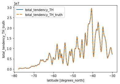
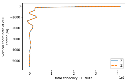
Now we do some checks to verify that the budget adds up.
We will take an average over the first 10 timesteps
time_slice = dict(time=slice(0, 10))
valid_range = dict(YC=slice(-90,-30))

def check_vertical(budget, suffix):
    ds_chk = (budget[[f'total_tendency_{suffix}', f'total_tendency_{suffix}_truth']]
              .sel(**valid_range).sum(dim=['Z', 'XC']).mean(dim='time'))
    return ds_chk

def check_horizontal(budget, suffix):
    ds_chk = (budget[[f'total_tendency_{suffix}', f'total_tendency_{suffix}_truth']]
              .sel(**valid_range).sum(dim=['YC', 'XC']).mean(dim='time'))
    return ds_chk
th_vert = check_vertical(budget_th.isel(**time_slice), 'TH').load()
th_vert.total_tendency_TH.plot(linewidth=2)
th_vert.total_tendency_TH_truth.plot(linestyle='--', linewidth=2)
plt.legend()
<matplotlib.legend.Legend at 0x7f10ba181240>
th_horiz = check_horizontal(budget_th.isel(**time_slice), 'TH').load()
th_horiz.total_tendency_TH.plot(linewidth=2, y='Z')
th_horiz.total_tendency_TH_truth.plot(linestyle='--', linewidth=2, y='Z')
plt.legend()
<matplotlib.legend.Legend at 0x7fe85f5ba470>
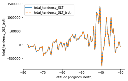
slt_vert = check_vertical(budget_slt.isel(**time_slice), 'SLT').load()
slt_vert.total_tendency_SLT.plot(linewidth=2)
slt_vert.total_tendency_SLT_truth.plot(linestyle='--', linewidth=2)
plt.legend()
<matplotlib.legend.Legend at 0x7f10b4ed7828>
slt_horiz = check_horizontal(budget_slt.isel(**time_slice), 'SLT').load()
slt_horiz.total_tendency_SLT.plot(linewidth=2, y='Z')
slt_horiz.total_tendency_SLT_truth.plot(linestyle='--', linewidth=2, y='Z')
plt.legend()
<matplotlib.legend.Legend at 0x7f10b3622160>
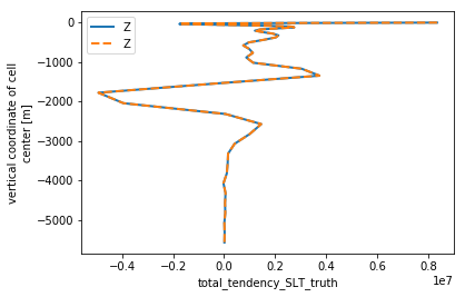
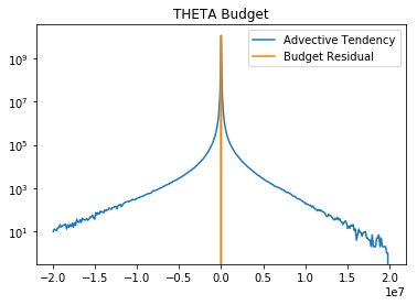
The curves look the same. But how do we know whether our error is truly “small”? Answer: we compare the distribution of the error
to the distribution of the other terms in the equation, e.g. \(P(G_{adv})\).
First we try to determine the appropriate range for our histograms by looking at the maximum values.
budget_th.isel(**time_slice).max().load()
<xarray.Dataset>
Dimensions:                  ()
Data variables:
    conv_horiz_adv_flux_TH   float32 19145940.0
    conv_horiz_diff_flux_TH  float32 89941.086
    conv_vert_adv_flux_TH    float32 23173650.0
    conv_vert_diff_flux_TH   float32 534407.7
    conv_total_flux_TH       float32 510076.62
    surface_flux_conv_TH     float32 21228.941
    lin_fs_correction_TH     float32 10248.496
    sw_flux_conv_TH          float32 21346.447
    total_tendency_TH        float32 510076.62
    total_tendency_TH_truth  float32 297048.4
budget_slt.isel(**time_slice).max().load()
<xarray.Dataset>
Dimensions:                   ()
Data variables:
    conv_horiz_adv_flux_SLT   float32 94174560.0
    conv_horiz_diff_flux_SLT  float32 17939.193
    conv_vert_adv_flux_SLT    float32 105942130.0
    conv_vert_diff_flux_SLT   float32 76532.33
    conv_total_flux_SLT       float32 5261500.5
    surface_flux_conv_SLT     float32 7828.6157
    lin_fs_correction_SLT     float32 20308.545
    total_tendency_SLT        float32 5261500.5
    total_tendency_SLT_truth  float32 46110.24
# parameters for histogram calculation
th_range = (-2e7, 2e7)
slt_range = (-1e8, 1e8)
valid_region = dict(YC=slice(-90, -30))
nbins = 301
# budget errors
error_th = budget_th.total_tendency_TH - budget_th.total_tendency_TH_truth
error_slt = budget_slt.total_tendency_SLT - budget_slt.total_tendency_SLT_truth
# calculate theta error histograms over the whole time range
adv_hist_th, hbins_th = dsa.histogram(budget_th.conv_horiz_adv_flux_TH.sel(**valid_region).data,
                                        bins=nbins, range=th_range)
err_hist_th, hbins_th = dsa.histogram(error_th.sel(**valid_region).data,
                                        bins=nbins, range=th_range)
err_hist_th, adv_hist_th = dask.compute(err_hist_th, adv_hist_th)
bin_c_th = 0.5*(hbins_th[:-1] + hbins_th[1:])
plt.semilogy(bin_c_th, adv_hist_th, label='Advective Tendency')
plt.semilogy(bin_c_th, err_hist_th, label='Budget Residual')
plt.legend()
plt.title('THETA Budget')
Text(0.5,1,'THETA Budget')
# calculate salt error histograms over the whole time range
adv_hist_slt, hbins_slt = dsa.histogram(budget_slt.conv_horiz_adv_flux_SLT.sel(**valid_region).data,
                                        bins=nbins, range=slt_range)
err_hist_slt, hbins_slt = dsa.histogram(error_slt.sel(**valid_region).fillna(-9e13).data,
                                        bins=nbins, range=slt_range)
err_hist_slt, adv_hist_slt = dask.compute(err_hist_slt, adv_hist_slt)
bin_c_slt = 0.5*(hbins_slt[:-1] + hbins_slt[1:])
plt.semilogy(bin_c_slt, adv_hist_slt, label='Advective Tendency')
plt.semilogy(bin_c_slt, err_hist_slt, label='Budget Residual')
plt.title('SALT Budget')
plt.legend()
<matplotlib.legend.Legend at 0x7f10a8201fd0>
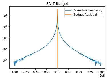
These figures show that the error is extremely small compared to the other terms in the budget.
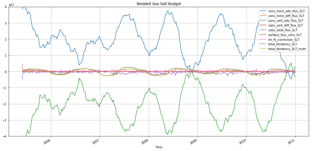
Finally, we can do some science: compute the salinity budget for a specific region, such as the upper Weddell Sea.
budget_slt_weddell = (budget_slt
                        .sel(YC=slice(-80, -68), XC=slice(290, 360), Z=slice(0, -500))
                        .sum(dim=('XC', 'YC', 'Z'))
                        .load())
budget_slt_weddell
<xarray.Dataset>
Dimensions:                   (time: 438)
Coordinates:
  * time                      (time) datetime64[ns] 2005-01-06 2005-01-11 ...
Data variables:
    conv_horiz_adv_flux_SLT   (time) float32 -43632460.0 -36267436.0 ...
    conv_horiz_diff_flux_SLT  (time) float32 4892.9424 6978.3486 10441.184 ...
    conv_vert_adv_flux_SLT    (time) float32 -110508056.0 56280100.0 ...
    conv_vert_diff_flux_SLT   (time) float32 4837898.5 -1010.3694 -1765.5066 ...
    conv_total_flux_SLT       (time) float32 -149297810.0 20018620.0 ...
    surface_flux_conv_SLT     (time) float32 -8284682.0 -3737431.2 ...
    lin_fs_correction_SLT     (time) float32 149588460.0 -17810290.0 ...
    total_tendency_SLT        (time) float32 -7993949.5 -1529094.9 ...
    total_tendency_SLT_truth  (time) float32 -7993943.5 -1529095.6 ...
plt.figure(figsize=(18,8))
for v in budget_slt_weddell.data_vars:
    budget_slt_weddell[v].rolling(time=30).mean().plot(label=v)
plt.ylim([-4e7, 4e7])
plt.legend()
plt.grid()
plt.title('Weddell Sea Salt Budget')
Text(0.5,1,'Weddell Sea Salt Budget')
plt.figure(figsize=(18,8))
for v in budget_slt_weddell.data_vars:
    budget_slt_weddell[v].rolling(time=30).mean().plot(label=v)
plt.ylim([-4e6, 4e6])
plt.legend()
plt.grid()
plt.title('Weddell Sea Salt Budget')
Text(0.5,1,'Weddell Sea Salt Budget')
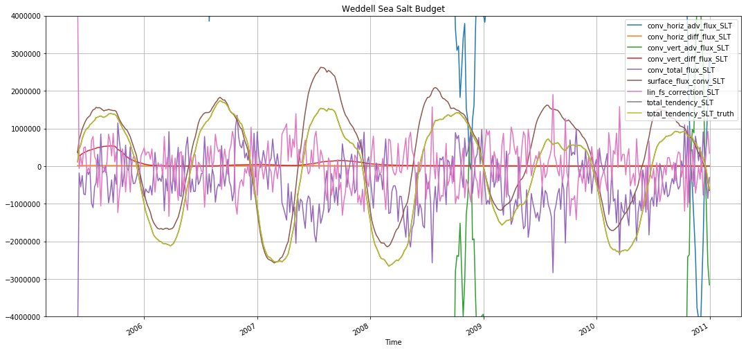
These figures show that, while they advective terms are the largest ones in the budget, the actual variability in salinity is driven primarily by the surface fluxes.
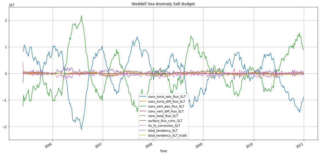
The timeseries is pretty short, but nevertheless we can try to remove the climatology to get a better idea of what drives the interannual variability
budget_slt_weddell_mm = budget_slt_weddell.groupby('time.month').mean(dim='time')
budget_slt_weddell_anom = budget_slt_weddell.groupby('time.month') - budget_slt_weddell_mm
plt.figure(figsize=(18,8))
for v in budget_slt_weddell.data_vars:
    budget_slt_weddell_anom[v].rolling(time=30).mean().plot(label=v)
plt.ylim([-2.5e7, 2.5e7])
plt.legend()
plt.grid()
plt.title('Weddell Sea Anomaly Salt Budget')
Text(0.5,1,'Weddell Sea Anomaly Salt Budget')
plt.figure(figsize=(18,8))
for v in budget_slt_weddell.data_vars:
    budget_slt_weddell_anom[v].rolling(time=30).mean().plot(label=v)
plt.ylim([-2.5e6, 2.5e6])
plt.legend()
plt.grid()
plt.title('Weddell Sea Anomaly Salt Budget')
Text(0.5,1,'Weddell Sea Anomaly Salt Budget')
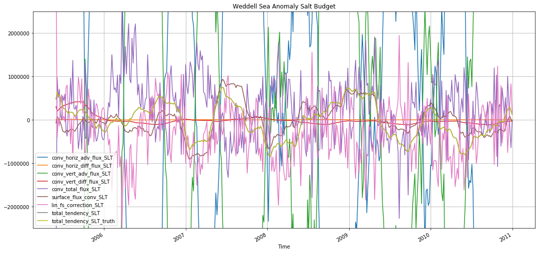
The monthly anomaly is also premoninantly driven by surface forcing.
Download python script: SOSE.py
Download Jupyter notebook: SOSE.ipynb